

For many manufacturing procurement teams, one of the most basic questions is also one of the hardest to answer confidently: where is our money actually going?
Direct materials purchasing spans multiple plants, dozens of categories, and often hundreds of suppliers. Data lives in different ERP systems. Supplier naming conventions aren’t standardized. Categories get classified differently depending on who entered the transaction. And nobody has time to reconcile it all manually.
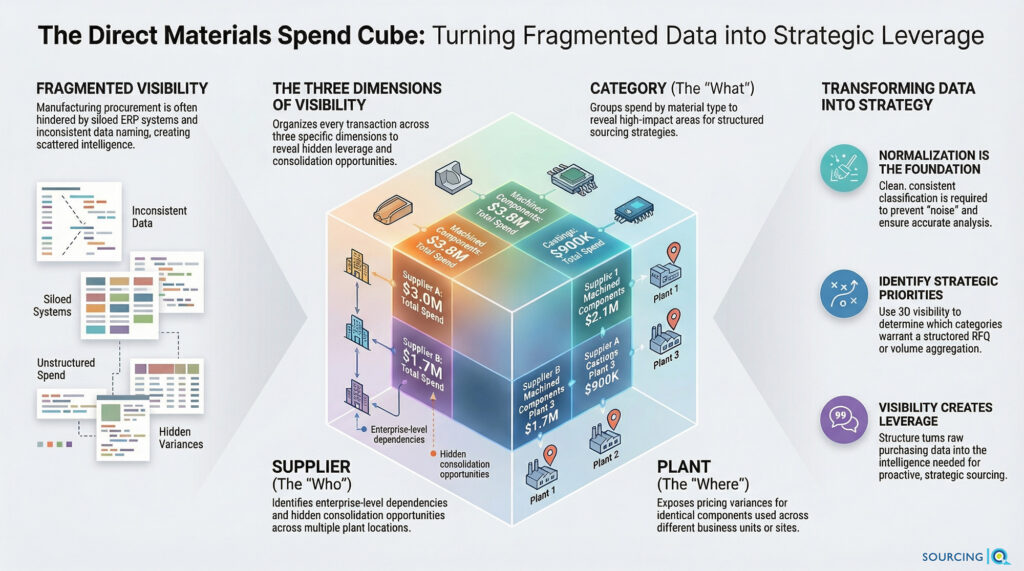
The result is fragmented visibility. Teams know their largest suppliers in broad strokes. They know roughly what they spend on steel or machined components. But they can’t easily see how purchasing patterns connect across the organization — which means consolidation opportunities stay invisible, leverage goes unrealized, and sourcing decisions stay reactive longer than they should.
This is exactly what a direct materials spend cube is built to solve.
What Is a Spend Cube?
A spend cube is a structured analytical model that organizes procurement data across three dimensions simultaneously, so you can analyze purchasing activity from multiple angles at once — not just one static report at a time.
The three dimensions are:
- Supplier — who you’re buying from
- Category — what you’re buying
- Business unit or plant — where you’re buying it
The “cube” metaphor works like this: each purchasing transaction sits at the intersection of all three dimensions. You can “slice” the data any direction — by supplier across all plants, by category across all suppliers, by plant across all categories — and each slice reveals something different.
That flexibility is where the analytical value lives.
The Three Dimensions in a Direct Materials Context
Supplier dimension
The supplier view answers concentration questions: who are you actually dependent on, and how much?
What tends to surface here:
- The same supplier quietly supporting multiple plants under different names in the system
- A handful of suppliers accounting for a disproportionate share of total spend
- Single-source situations that nobody deliberately chose — they just accumulated
- Consolidation opportunities that are invisible plant-by-plant but obvious at the enterprise level
Many manufacturers discover through this view that they’re already doing significant business with a supplier across multiple sites — but buying as if they were three small customers instead of one large one. That’s leverage left on the table.
Category dimension
The category view groups purchasing by material or component type. In direct materials, that typically looks like:
- Machined components
- Castings and forgings
- Fabricated metal parts
- Electronics and electrical assemblies
- Plastics and molded components
- Packaging
Good category classification is what determines whether this dimension is useful or just noise. If machined components appear in the data as “CNC part,” “precision metal component,” “machined assembly,” and “turned part” — all filed under different line items — the category view won’t show you what you’re actually spending on machined components. It’ll show you four unrelated buckets.
This is why classification is the most important (and most labor-intensive) step in building a spend cube. The quality of the categories determines the quality of every insight that follows.
Once categories are clean, the dimension reveals which ones are high-spend, which have fragmented supplier bases worth consolidating, and which are large enough to warrant a structured sourcing strategy.
Plant or business unit dimension
Manufacturing organizations rarely buy as a single entity. Procurement is distributed across plants, divisions, and product lines — often with minimal coordination between them.
The plant dimension makes that visible. The same category, analyzed across facilities, frequently reveals:
- Different suppliers used for functionally identical components
- Pricing variance for the same material across sites
- One plant single-sourced where another has two qualified vendors
- Volume fragmented across sites that, if aggregated, would create real leverage
Without this cross-plant view, these patterns stay hidden inside local buying decisions. The spend cube brings them to the surface.
A Spend Cube Example in Practice
Here’s a simplified illustration of what spend cube data looks like and what it reveals:
| Supplier | Category | Plant | Annual Spend |
| Supplier A | Machined Components | Plant 1 | $2.1M |
| Supplier B | Machined Components | Plant 2 | $1.7M |
| Supplier A | Castings | Plant 3 | $900K |
| Supplier C | Plastics | Plant 1 | $1.2M |
| Supplier B | Castings | Plant 2 | $750K |
Run this through the three dimensions and here’s what you start to see:
Supplier view: Supplier A is active across two categories and two plants. Supplier B shows up in two categories at Plant 2. Neither relationship has likely been managed as an enterprise account — which means pricing, terms, and performance expectations are probably inconsistent.
Category view: Machined components represent the largest spend category in the sample. Are both plants buying to the same spec? Are the suppliers aware they’re competing for the same company’s volume? Probably not.
Plant view: Plants 1 and 2 are both buying castings — from different suppliers, likely at different prices, under different terms. That’s a cross-plant sourcing conversation waiting to happen.
None of this is visible in a standard ERP report sorted by supplier or PO number. The cube structure makes it obvious.
Building the Dataset: What You Actually Need
You don’t need a sophisticated tool to build a working spend cube. You need clean, structured data. The core fields:
- Supplier name (normalized — one supplier shouldn’t appear as five)
- Category classification (consistent, manufacturing-relevant buckets)
- Plant or business unit
- Purchase amount
- Item description and part number
- Date of purchase
The normalization step is where most teams get stuck. Raw ERP data has inconsistent supplier names, vague item descriptions, and category codes designed for accounting rather than procurement analysis. Before any meaningful analysis can happen, that data needs to be cleaned and reclassified into categories that reflect how manufacturing actually works — not how the chart of accounts was set up in 2009.
It’s tedious work. It’s also what separates a spend cube that generates real insight from one that just produces a prettier version of the confusion you already had.
Why This Matters for Strategic Sourcing
Spend cubes aren’t reporting artifacts. They’re the analytical foundation that strategic sourcing decisions are built on.
With structured spend visibility across all three dimensions, procurement teams can identify:
- Which supplier relationships are worth investing in — and which are accidental
- Which categories are large enough and competitive enough to warrant a structured RFQ
- Where cross-plant volume aggregation creates pricing leverage
- Where single-source concentration is creating risk nobody’s managing
- Which cost reduction initiatives are worth pursuing first
Without this visibility, sourcing strategy is driven by urgency and familiarity — whoever yells loudest or whoever procurement has always used. With it, strategy can be driven by impact and feasibility.
This is why most procurement transformations start with spend analysis. You can’t prioritize what you can’t see.
Structure Creates Visibility. Visibility Creates Leverage.
Manufacturing procurement environments are inherently complex — and complexity hides cost. Multiple plants, varied components, fragmented data systems, and decentralized buying behavior all work against the kind of visibility that enables smart sourcing decisions.
The direct materials spend cube doesn’t eliminate that complexity. It organizes it into something actionable: a structured view of who you’re buying from, what you’re buying, and where you’re buying it — simultaneously.
That structure is what turns raw purchasing data into procurement intelligence. And procurement intelligence is what separates reactive buying from strategic sourcing.